Colours

The default palette

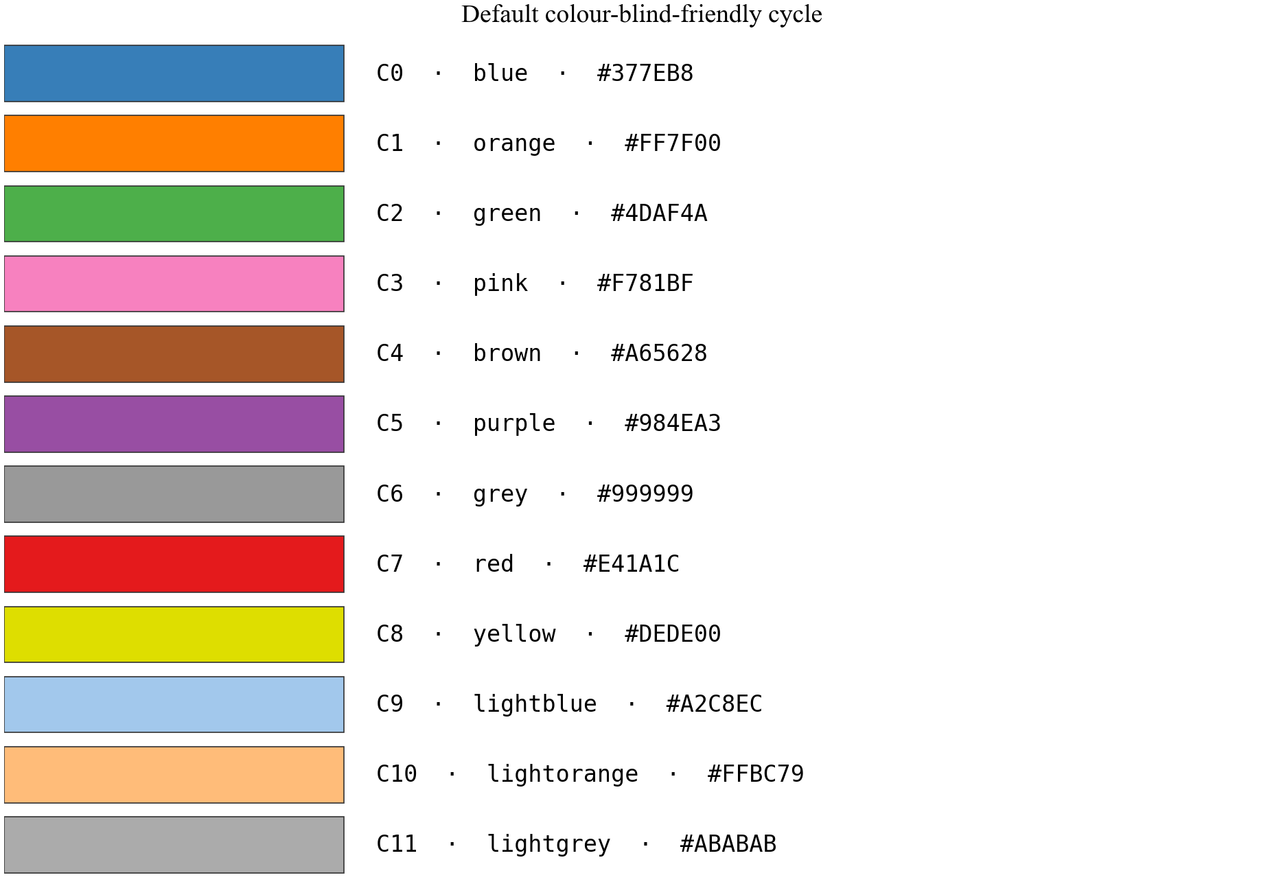
The default cycle has 12 colours, all accessible by name via plotastro.COLORS (e.g. pa.COLORS["blue"]), or as matplotlib’s "C0"…"C11" shorthands:

• C0–C8 are a colour-blind-safe re-ordering of the ColorBrewer Set1 qualitative palette (popularised by Thøger Rivera-Thorsen’s CBcycle). Consecutive colours differ in lightness as well as hue, so adjacent lines stay distinguishable under the common deficiencies (deuteranopia, protanopia) and in greyscale print; the notorious red–green pair is pushed far apart in the cycle (green is C2, red is C7), so plots with a handful of lines never rely on it.

• C9–C11 are light companions (from Tableau’s Color Blind 10): use them for uncertainty bands, reference curves, or de-emphasised data underneath a saturated line of the same hue.

Matched shades without transparency

Better for print and EPS than alpha= (no colour shifts where elements overlap):

ax.plot(x, y, color=pa.COLORS["blue"])
ax.fill_between(x, lo, hi, color=pa.lighten(pa.COLORS["blue"], 0.7))
pa.darken(pa.COLORS["orange"], 0.3)     # the other direction

More palettes

• pa.OKABE_ITO — Okabe & Ito (2008), the classic CVD-safe recommendation for categorical colours in science;

• pa.PETROFF10 — Petroff (2021), the CVD-optimised 10-colour cycle used across particle physics;

• pa.PETROFF8 — Petroff’s 8-colour sibling, the default cycle of the Euclid Consortium’s niceplots (and of the euclid style here);

• pa.TOL_VIBRANT — Paul Tol’s vibrant qualitative scheme, 7 CVD-safe colours;

• pa.PAIRED — light/dark pairs for data/model or before/after comparisons: pa.PAIRED["blue"] → ("#a6cee3", "#1f78b4").

Any of them can become the active cycle when you activate a style — pa.set_style("mnras", palette="okabe_ito") — or pass your own list of colours.

Euclid colour schemes

The euclid style (see Supported journals) and these colour schemes are adapted from the Euclid Consortium Editorial Board’s niceplots (Euclid-internal, GPL-3.0): the colours are re-expressed here, nothing is copied from it. plotastro.euclid_colors() returns each scheme under its niceplots name:

scheme	colours
"categorical1"	Petroff (2021) 8 colours — pa.PETROFF8; the Euclid default
"categorical2"	Okabe & Ito — pa.OKABE_ITO
"categorical3"	black, then Tol’s vibrant scheme — pa.TOL_VIBRANT
"sequential"	n colours of increasing brightness from copper
"diverging"	n colours from blue to red from coolwarm

pa.set_style("euclid", palette="categorical3")                 # by name
ax.set_prop_cycle(color=pa.euclid_colors("sequential", n=6))   # per axes

Checking accessibility yourself

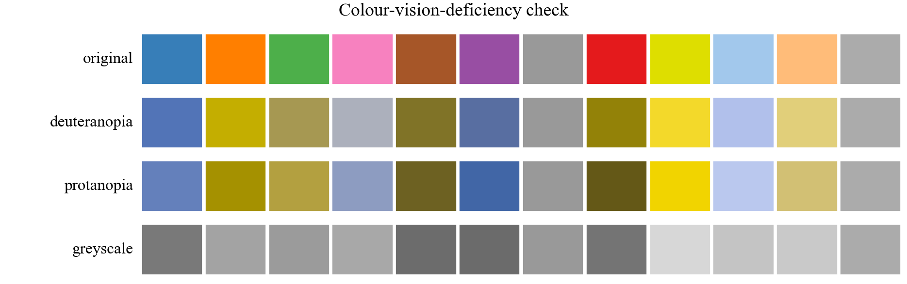
Don’t take the palette’s word for it — simulate it (Machado et al. 2009 model, no extra dependencies):

pa.check_colors()                 # any palette under deuteranopia/protanopia/greyscale
pa.check_colors(pa.PAIRED)        # works on your own colour lists/dicts too
pa.check_figure(fig)              # simulate a whole rendered figure — the
                                  # final check before submission
pa.simulate_cvd("#e41a1c", "deuteranopia")   # the raw transform

If two lines merge in any panel, add markers or dash patterns (see Markers, line styles and panel labels), or pick colours further apart in the cycle. MNRAS recommends Color Oracle and ColorBrewer for exactly this; with plotastro it’s built in.

Colormaps

The styles default to viridis (perceptually uniform, CVD-safe). Good picks: viridis/magma/cividis for sequential data, RdBu_r or coolwarm for diverging data (red–blue, not red–green). Avoid jet/rainbow. To change the default for every imshow, pcolormesh, scatter, … pass cmap= when you activate a style:

pa.set_style("mnras", cmap="cividis")

For many more maps, plotastro can use CMasher (next section); see also cmocean.

CMasher colours and colormaps (optional)

CMasher (van der Velden 2020, JOSS 5, 2004) is a collection of scientific colormaps: sequential, diverging and cyclic, all designed to be perceptually uniform, and most of them colour-vision-deficiency friendly. plotastro can use them for discrete colours and for colormaps. CMasher is not a dependency of plotastro: install it only if you want it,

pip install cmasher                # or: pip install "plotastro[cmasher]"

and plotastro imports it only when you ask for a CMasher colour. Every other feature works the same without it.

Five ways to use it

you want	write
a colour cycle for every figure	pa.set_style("mnras", palette="cmr.rainforest")
a default colormap for every figure	pa.set_style("mnras", cmap="cmr.ocean")
n colours, e.g. one per line	pa.cmasher_colors("torch", n=5)
a colormap, optionally cut or split into levels	pa.cmasher_cmap("iceburn", cmap_range=(0.1, 0.9), n=6)
a map by name in any matplotlib call	cmap="cmr.iceburn" (once CMasher is imported)

CMasher names start with cmr., which is also how its maps are registered with matplotlib. plotastro.cmasher_colors() and plotastro.cmasher_cmap() accept names with or without the prefix ("torch" or "cmr.torch"), but set_style(palette=..., cmap=...) and matplotlib need the cmr. prefix. Add _r to any name for the reversed map: "cmr.rainforest_r".

Choosing a map

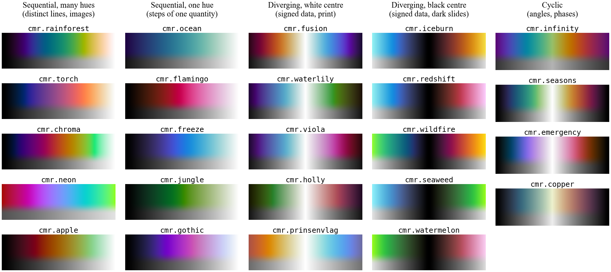
Pick the type of map from the kind of data, then a map from that group. The figure shows each map in colour, with its greyscale version (what a black-and-white printout shows) underneath.

data	type of map	try
lines that must be easy to tell apart; images	sequential, many hues	rainforest, torch, chroma, neon, apple
steps of one quantity: redshift, mass, time, …	sequential, one hue	ocean, flamingo, freeze, jungle, gothic
signed data around a reference value: residuals, over/under-densities, velocities	diverging	white centre: fusion, waterlily, viola, holly, prinsenvlag; black centre: iceburn, redshift, wildfire, seaweed, watermelon
angles, phases, directions	cyclic	infinity, seasons, emergency, copper

Things to know when choosing:

• Sequential maps survive greyscale. In every CMasher sequential map the lightness rises steadily from one end to the other, so the order of the colours is still readable in black and white.

• Diverging maps lose the sign in greyscale. Their lightness is the same at equal distances either side of the centre, so +x and -x look alike in black and white. If the sign matters in print, add contours or say so in the caption.

• White or black centre. A white centre fades values near zero into the page, which suits print. A black centre makes the extremes the brightest colours, which stands out on dark backgrounds such as slides.

• Cyclic maps start and end on the same colour, so -180° and +180° match. Each has a version shifted by half a cycle, with _s at the end of the name. For example, seasons is white at the centre of the range and black at its ends, and seasons_s is the other way round.

• Every map: cmasher.get_cmap_list("sequential") (or "diverging", "cyclic") lists all of them, and cmasher.view_cmap("cmr.torch", show_grayscale=True) previews one. The CMasher documentation shows them all.

Discrete colours

Pass a "cmr." name as the palette to get a colour cycle of 8 colours sampled from that map, or use plotastro.cmasher_colors() for a different number:

pa.set_style("mnras", palette="cmr.rainforest")              # 8-colour cycle
ax.set_prop_cycle(color=pa.cmasher_colors("torch", n=5))     # 5, this axes only
colors = pa.cmasher_colors("ocean", n=4, cmap_range=(0.2, 0.8))

The colours are hex strings, equally spaced over cmap_range. Its default, (0.15, 0.85), follows CMasher’s own advice: most of its sequential maps run from black to white, and those ends disappear against the axes or the page.

These cycles are ordered from dark to light, and a matplotlib cycle starts at the first colour. So for a fixed number of lines, sample exactly that many and they will span the whole map. A family of models at several redshifts:

redshifts = [0, 0.5, 1, 2]
colors = pa.cmasher_colors("ocean", n=len(redshifts))

fig, ax = pa.subplots()
for z, color in zip(redshifts, colors):
    ax.loglog(k, pk(k, z), color=color, label=f"$z = {z}$")
ax.legend()

Because the colours are plain hex strings, they work anywhere matplotlib takes a colour. You can also pass them to plotastro.lighten() for a matching uncertainty band:

for z, color in zip(redshifts, colors):
    ax.plot(k, pk(k, z), color=color)
    ax.fill_between(k, lo(k, z), hi(k, z), color=pa.lighten(color, 0.6))

pa.lighten keeps a colour’s saturation, so the near-black end of a map turns into a strong, bright shade. For bands, start the range above the darkest end, e.g. cmap_range=(0.3, 0.8).

More recipes:

• Add markers so the lines also differ in greyscale. Build the cycle with plt.cycler; plotastro.style_cycler() always uses the default palette.

  colors = pa.cmasher_colors("torch", n=4)
  ax.set_prop_cycle(plt.cycler(color=colors) + plt.cycler(marker=pa.MARKERS[:4]))
  

• Reverse the order (light to dark) with _r: pa.cmasher_colors("ocean_r", n=4).

• On a dark background, such as dark slides, keep to the light part of the map: pa.cmasher_colors("ocean", n=4, cmap_range=(0.4, 1.0)).

• Check the result with pa.check_colors(colors), as for any other palette.

Colormaps

Make a CMasher map the default colormap with set_style(cmap=...), or get the colormap itself with plotastro.cmasher_cmap(). It can also cut the map to part of its range, or split it into a few discrete levels:

pa.set_style("mnras", cmap="cmr.ocean")            # default for imshow etc.

ax.imshow(img, cmap=pa.cmasher_cmap("rainforest"))
ax.pcolormesh(x, y, z, cmap=pa.cmasher_cmap("ocean", cmap_range=(0.15, 0.85)))
ax.contourf(x, y, z, levels=6, cmap=pa.cmasher_cmap("iceburn", n=6))

Once CMasher has been imported (by plotastro or by import cmasher), every matplotlib function also accepts its maps by name: cmap="cmr.iceburn".

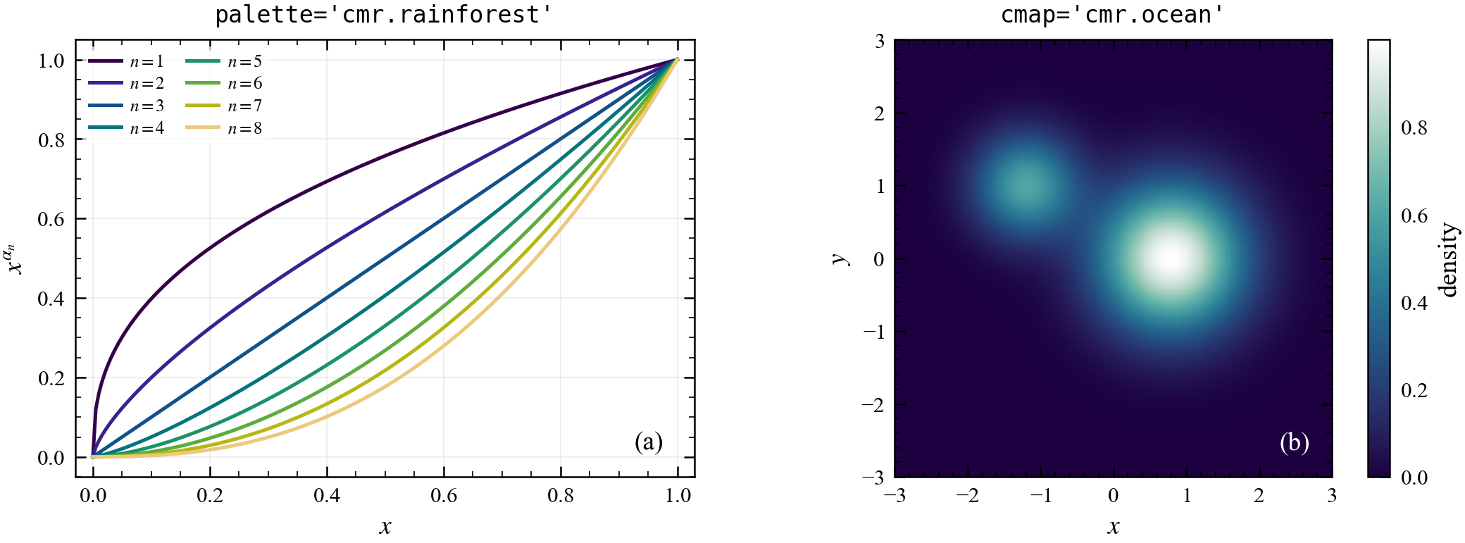
The four common cases, as in the figure below:

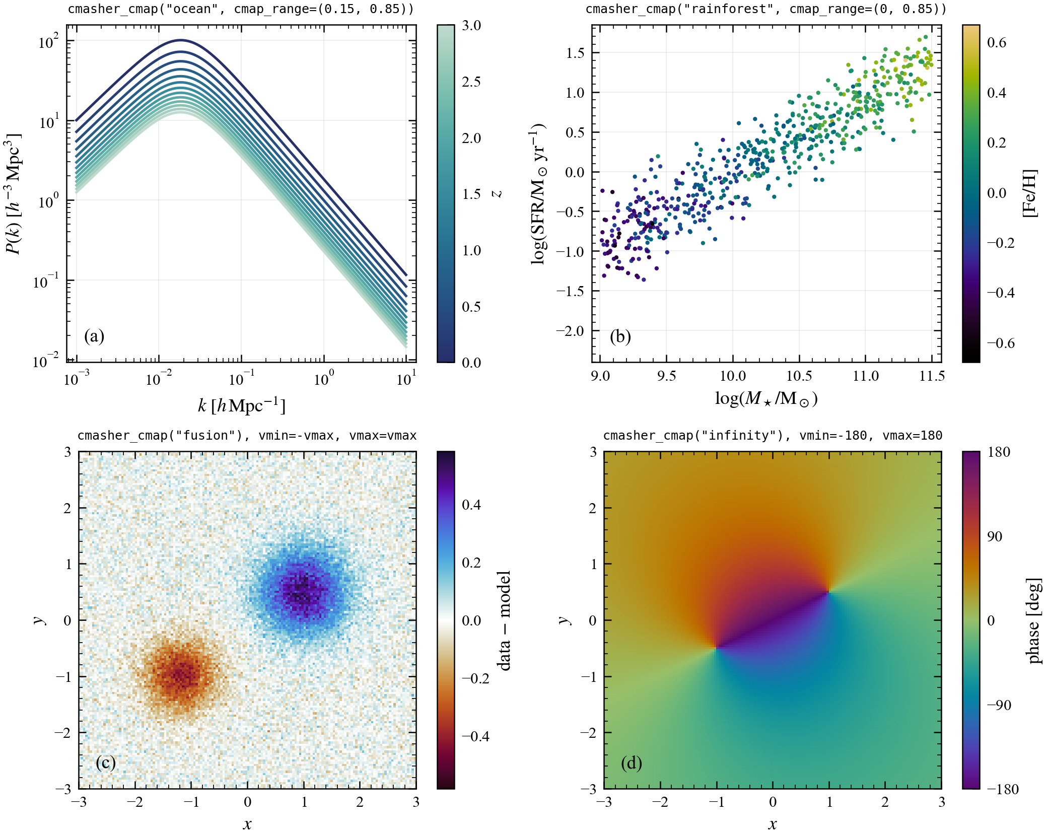
(a) Many lines coloured by a continuous parameter. With a dozen or more lines, a colour bar is clearer than a legend. Take the line colours from the same colormap and normalisation that you give the colour bar, so the two match:

import matplotlib as mpl

redshifts = np.linspace(0, 3, 13)
cmap = pa.cmasher_cmap("ocean", cmap_range=(0.15, 0.85))
norm = mpl.colors.Normalize(redshifts.min(), redshifts.max())

fig, ax = pa.subplots()
for z in redshifts:
    ax.loglog(k, pk(k, z), color=cmap(norm(z)))
fig.colorbar(mpl.cm.ScalarMappable(norm=norm, cmap=cmap), ax=ax, label="$z$")

(b) Points coloured by a third quantity. Cut off the white end of a sequential map, so that no point fades into the page:

sc = ax.scatter(logm, sfr, c=metallicity, s=4,
                cmap=pa.cmasher_cmap("rainforest", cmap_range=(0, 0.85)))
fig.colorbar(sc, ax=ax, label=r"$[\mathrm{Fe/H}]$")

(c) Signed data on a diverging map. Make the limits symmetric, so that zero falls on the centre of the map:

vmax = np.abs(residual).max()
im = ax.imshow(residual, origin="lower", cmap=pa.cmasher_cmap("fusion"),
               vmin=-vmax, vmax=vmax)
fig.colorbar(im, ax=ax, label="data $-$ model")

norm=mpl.colors.CenteredNorm() does the same without computing vmax yourself.

(d) An angle on a cyclic map. Set the limits to one full period, so that the colour wraps around exactly:

im = ax.imshow(phase_deg, origin="lower", cmap=pa.cmasher_cmap("infinity"),
               vmin=-180, vmax=180)
fig.colorbar(im, ax=ax, label="phase [deg]", ticks=[-180, -90, 0, 90, 180])

Two more options of plotastro.cmasher_cmap():

• Discrete levels, with n=. For filled contours, set n to the number of bands, which is one fewer than the number of level edges. Each band then gets one colour of the map, and the colour bar shows the same steps:

  levels = np.linspace(-1, 1, 6)                     # 6 edges -> 5 bands
  cs = ax.contourf(x, y, z, levels=levels, cmap=pa.cmasher_cmap("fusion", n=5))
  fig.colorbar(cs, ax=ax)
  

• Part of a map, with cmap_range=. Use it, for example, to drop a black end that would merge with an image’s empty background: pa.cmasher_cmap("ocean", cmap_range=(0.1, 1.0)). CMasher advises keeping at least half of a sequential map, so that it stays smooth.

One choice for a whole paper

Set the colours and the colormap once, when you activate the style. Every figure after that uses them:

pa.set_style("mnras", palette="cmr.rainforest", cmap="cmr.ocean")

Before submitting, check the finished figures with pa.check_figure(fig) (see Checking accessibility yourself).

Co-authors without CMasher

Discrete colours are plain hex strings. To let a script run without CMasher installed, print the colours once and paste the list in its place:

print(pa.cmasher_colors("rainforest"))
# ['#...', '#...', ...]   -> pa.set_style("mnras", palette=[...that list...])

Colormaps can’t be pasted in like this. Anyone running the colormap code needs CMasher installed.

Troubleshooting

ImportError: This feature needs the optional CMasher package

CMasher isn’t installed in the environment you’re running: pip install cmasher.

ValueError: 'cmr.ocean' is not a valid value for cmap (from matplotlib)

CMasher hasn’t been imported yet in this session, so matplotlib doesn’t know the cmr. names. Any plotastro CMasher call imports it, or add import cmasher at the top of the script. Passing cmap=pa.cmasher_cmap("ocean") instead of the name also works.

ValueError: Unknown CMasher colormap '...'

The name is misspelled, or isn’t in your CMasher version. cmasher.get_cmap_list() lists the maps you have.

ValueError: Unknown palette 'rainforest'

set_style(palette=...) needs the cmr. prefix: palette="cmr.rainforest".

If you use CMasher in a paper, please cite it; cmasher.get_bibtex() prints the reference.